A model is considered linear if the transformation of features that is used to calculate the prediction is a linear combination of the features. The possibilities for a linear combination are that each feature can be multiplied by a numerical constant, these terms can be added together, and an additional constant can be added. For example, in a simple model with two features, X1 and X2, a linear combination would take the form:

Linear combination of X1 and X2

The constants i, can be any number, positive, negative, or zero, for i = 0, 1, and 2 (although if a coefficient is 0, this removes a feature from the linear combination). A familiar example of a linear transformation of one variable is a straight line with the equation y = mx + b. In this case, o = b and 1 = m. o is called the intercept of a linear combination, which should make sense when thinking about the equation of a straight line in slope-intercept form like this.

However, while these transformations are not part of the basic formulation of a linear combination, they could be added to a linear model by engineering features, for example defining a new feature, X3 = X12.

Predictions of logistic regression, which take the form of probabilities, are made using the sigmoid function. This function is clearly non-linear and is given by the following:

 

Non-linear sigmoid function

Why, then, is logistic regression considered a linear model? It turns out that the answer to this question lies in a different formulation of the sigmoid equation, called the logit function. We can derive the logic function by solving the sigmoid function for X; in other words, finding the inverse of the sigmoid function. First, we set the sigmoid equal to p, the probability of observing the positive class, then solve for X as shown in the following:

 

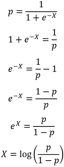
Solving for X

Here, we’ve used some laws of exponents and logs to solve for X. You may also see the logit expressed as:

 

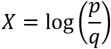
Logit function

The probability of failure, q, is expressed in terms of the probability of success, p: q = 1 – p, because probabilities sum to 1. Even though in our case, credit default would probably be considered a failure in the sense of real-world outcomes, the positive outcome (response variable = 1 in a binary problem) is conventionally considered “success” in mathematical terminology. The logit function is also called the log odds, because it is the natural logarithm of the odds ratio, p/q. Odds ratios may be familiar from the world of gambling, via phrases such as “the odds are 2 to 1 that team a defeats team b.”

In general, what we’ve called capital X in these manipulations can stand for a linear combination of all the features. For example, this would be X = o + 1X1 + 2X2 in our simple case of two features. Logistic regression is considered a linear model because the features included in X are, in fact, only subject to a linear combination when the response variable is considered to be the log odds. This is an alternative way of formulating the problem, as compared to the sigmoid equation.

In summary, the features X1, X2,…, Xj look like this in the sigmoid equation version of logistic regression:

 

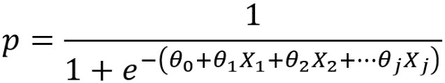
Sigmoid version of logistic regression

But they look like this in the log odds version, which is why logistic regression is called a linear model:

 

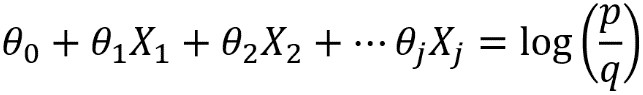
Log odds version of logistic regression

Because of this way of looking at logistic regression, ideally the features of a logistic regression model would be linear in the log odds of the response variable.