Packt Humble Bundle package

I am pleased to announce that my title, Python Machine Learning Cookbook, is part of the Packt Humble Bundle package, currently on sale on the Humble Bundle website until May 27, 2019.

PMLC

Humble Bundle is a distribution platform that sells games, ebooks, software, and other digital content. Since their inception in 2010, their mission has been to support charities (“Humble”) while providing awesome content to customers at great prices (“Bundle”). So far they helped to raise of $140m for a number of featured charities.

www.humblebundle.com

Keras 2.x Projects

9 projects demonstrating faster experimentation of neural network and deep learning applications using Keras.

Keras 2.x Projects explains how to leverage the power of Keras to build and train state-ofthe-
art deep learning models through a series of practical projects that look at a range of
real-world application areas.

To begin with, you will quickly set up a deep learning environment by installing the Keras
library. Through each of the projects, you will explore and learn the advanced concepts of
deep learning and will learn how to compute and run your deep learning models using the
advanced offerings of Keras. You will train fully-connected multilayer networks,
convolutional neural networks, recurrent neural networks, autoencoders and generative
adversarial networks using real-world training datasets. The projects you will undertake
are all based on real-world scenarios of all complexity levels, covering topics such as
language recognition, stock volatility, energy consumption prediction, faster object
classification for self-driving vehicles, and more.

Keras2.xProjects

By the end of this book, you will be well versed with deep learning and its implementation
with Keras. You will have all the knowledge you need to train your own deep learning
models to solve different kinds of problems.

Keras 2.x Projects

Keras Reinforcement Learning Projects

9 projects exploring popular reinforcement learning techniques to build self-learning agents

Reinforcement learning has evolved a lot in the last couple of years and proven to be a successful technique in building smart and intelligent AI networks. Keras Reinforcement Learning Projects installs human-level performance into your applications using algorithms and techniques of reinforcement learning, coupled with Keras, a faster experimental library. In the following the link at the book:

kerasrlsmall

The book begins with getting you up and running with the concepts of reinforcement learning using Keras. You’ll learn how to simulate a random walk using Markov chains and select the best portfolio using dynamic programming (DP) and Python. You’ll also explore projects such as forecasting stock prices using Monte Carlo methods, delivering vehicle routing application using Temporal Distance (TD) learning algorithms, and balancing a Rotating Mechanical System using Markov decision processes.

Once you’ve understood the basics, you’ll move on to Modeling of a Segway, running a robot control system using deep reinforcement learning, and building a handwritten digit recognition model in Python using an image dataset. Finally, you’ll excel in playing the board game Go with the help of Q-Learning and reinforcement learning algorithms.

By the end of this book, you’ll not only have developed hands-on training on concepts, algorithms, and techniques of reinforcement learning but also be all set to explore the world of AI.

Why is OOP in R so confusing?

Author: Omar Trejo Navarro

Apart from the fact that R is an interpreted language, which can pretty much confuse people used to compiled languages, most programmers would agree that manipulating objects in R can sometimes be a nightmare. This has to do with two significant features of R that make OOP manipulation highly efficient:

  • R has several object models unlike Java, Python and others, which have only one
  • R implements parametric polymorphism, while other OOP (Object-oriented programming) languages generally implement polymorphism from inside an object

Let’s look at these two in a bit more detail.

Various object models

Working with OOP in R is different from what you may see in other languages such as Python, Java, C++, etc. These languages have a single object model. However, R has various object models, meaning that it lets us implement object-oriented systems in various ways. Specifically, R has the following object models:

  • S3
  • S4
  • Reference Classes
  • R6
  • Base Types

OOP1

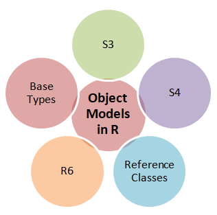
In this article, we will look at S3, S4, and R6, since these are the most-used object models in R, but more on that later. Let’s first understand what parametric polymorphism is.

Parametric polymorphism

R implements parametric polymorphism, which implies that methods in R belong to functions, not classes. Parametric polymorphism basically lets you define a generic method or function for types of objects you haven’t yet defined and may never do. This means that you can use the same name for several functions with different sets of arguments and from various classes.

R’s method calls look just like function calls and R must have a mechanism to know which names require simple function calls and which names require method calls. This mechanism is called generics. Generics allow you to register certain names to be treated as methods in R, and they act as dispatchers. When these registered generic functions are called, R looks into a chain of attributes in the object being passed in the call in order to look for functions that match the method call for that object’s type. If it finds a function, it will call it.

You may have noted that the plot() and summary() functions in R may return different results depending on the objects being passed to them (e.g. a data frame or a linear model instance). This is because they are generic functions that implement polymorphism. This way of working provides simple interfaces for users and makes their tasks much simpler. For instance, if you are exploring a new package and you get some kind of result at some point derived from the package, try calling plot(result), and you may be surprised to get some kind of plot that makes sense. This is not common in other OOP languages.

Now that we have a basic idea of what parametric polymorphism is and how it sets R apart from other OOP languages, let’s look at S3, S4, and R6.

R’s most common object models

The S3 object model of R owes its roots to the object model of the S language, the predecessor of R. S’s object model evolved over time, and its third version introduced class attributes, which paved the way for S3. S3 is the fundamental object model of R, and many of R’s own built-in classes are of the S3 type.

Being the least formal object model in R, S3 does lack in some key respects:

  • It has no formal class definitions, thereby leaving no scope for inheritance or encapsulation
  • Polymorphism can only be implemented through generics

Nevertheless, it makes up for what it lacks in by providing quite a lot of flexibility to the programmers. In the words of Hadley Wickham, “S3 has a certain elegance in its minimalism: you can’t take away any part of it and still have a useful object-oriented system“.

However, one of the biggest demerits of S3 is that it doesn’t provide the required safety; it is very easy to create a class in S3, but it may lead to very confusing and hard-to-debug code if not used with utmost care. For example, a programmer could misspell a function and S3 would raise no issues. This is why S4 came into the picture, developed with the goal of adding safety. It keeps the code safe but, on the flip side, introduces a lot of verbosity to the code. It implements most features of modern object-oriented programming languages:

  • Formal class definitions
  • Inheritance
  • Polymorphism (parametric)
  • Encapsulation

In reality, S3 and S4 are really just ways to implement polymorphism for static functions. The R6 package provides a type of class that is similar to R’s Reference Classes, but it is more efficient and doesn’t depend on S4 classes and the methods package, as Reference Classes do.

When Reference Classes were introduced, some users called the new class system R5, following the names of R’s existing class systems S3 and S4. Although Reference Classes are not actually called R5 nowadays, the name of this package and its classes follow the pattern. Despite being first released over 3 years ago, R6 isn’t widely known. However, it is widely used. For example, R6 is used within Shiny and to manage database connections in the dplyr package.

The decision of which object model to use eventually boils down to a trade-off between flexibility, formality and code cleanness.

R Programming by Example

R is a high-level statistical language and is widely used among statisticians and data miners to develop analytical applications. Given the obvious advantages that R brings to the table, it has become imperative for data scientists to learn the essentials of the language.

R Programming by Example is a hands-on guide that helps you develop a strong fundamental base in R by taking you through a series of illustrations and examples. Written by Omar Trejo Navarro, the book starts with the basic concepts and gradually progresses towards more advanced concepts to give you a holistic view of R. Omar is a well-respected data consultant with expertise in applied mathematics and economics.

If you are an aspiring data science professional or statistician and want to learn more about R programming in a practical and engaging manner, R Programming by Example is the book for you!

OOP2

Regression Analysis with R

Design and develop statistical nodes to identify unique relationships within data at scale

Regression analysis is a statistical process which enables prediction of relationships between variables. The predictions are based on the casual effect of one variable upon another. Regression techniques for modeling and analyzing are employed on large set of data in order to reveal hidden relationship among the variables.

Regression Analysis with R

This book will give you a rundown explaining what regression analysis is, explaining you the process from scratch. The first few chapters give an understanding of what the different types of learning are – supervised and unsupervised, how these learnings differ from each other. We then move to covering the supervised learning in details covering the various aspects of regression analysis. The outline of chapters are arranged in a way that gives a feel of all the steps covered in a data science process – loading the training dataset, handling missing values, EDA on the dataset, transformations and feature engineering, model building, assessing the model fitting and performance, and finally making predictions on unseen datasets. Each chapter starts with explaining the theoretical concepts and once the reader gets comfortable with the theory, we move to the practical examples to support the understanding. The practical examples are illustrated using R code including the different packages in R such as R Stats, Caret and so on. Each chapter is a mix of theory and practical examples.

By the end of this book you will know all the concepts and pain-points related to regression analysis, and you will be able to implement your learning in your projects.

Regression Analysis with R

Tipi di variabili in R

python

In questo post approfondiremo il concetto di variabili in ambiente R fornendo una spiegazione sulle differenti tipologie di variabili.Il linguaggio R prevede due tipi di variabili:

1)     variabili globali;

2)     variabili locali;

Come si può intuire, le variabili globali sono accessibili a livello globale all’interno del programma, le variabili locali invece assumono significato solo ed esclusivamente nel settore di appartenenza, risultando visibili solo all’interno del metodo in cui vengono inizializzate.

Per la maggior parte dei compilatori, un nome di variabile può contenere fino a trentuno caratteri, in modo da poter adottare per una variabile un nome sufficientemente descrittivo, in R tale limite non è indicato. La scelta del nome assume un’importanza fondamentale al fine di rendere leggibile il codice; questo perché un codice leggibile sarà facilmente mantenibile anche da persone diverse dal programmatore che l’ha creato.

Abbiamo parlato d’inizializzazione della variabile intesa quale operazione di creazione della variabile; vediamone allora un esempio banale:

> a <- 1

In tale istruzione è stato utilizzato l’operatore di assegnazione (<-), con il significato di assegnare appunto alla locazione di memoria individuata dal nome a il valore 1. Il tipo attribuito alla variabile è stabilito in fase d’inizializzazione; sarà allora che si deciderà se assegnare a essa una stringa di testo, un valore booleano (true/false), un numero decimale etc.

Per approfondire l’argomento:


Variabili ed espressioni in R

python

Le Variabili ed espressioni in R sono trattate in modo moderno ed efficiente, infatti mentre nella maggior parte dei linguaggi di programmazione è necessaria una dichiarazione delle variabili utilizzate all’interno del programma, dichiarazione effettuata nella parte iniziale prima della sezione esecutiva dello stesso, in R tutto questo non è richiesto. Poiché il linguaggio non richiede la dichiarazione delle variabili; il tipo e la relativa dimensione saranno decisi nel momento in cui le stesse saranno inizializzate.

Con il termine variabile ci si riferisce a un tipo di dato il cui valore è variabile nel corso dell’esecuzione del programma. È però possibile assegnarne un valore iniziale, si parlerà allora d’inizializzazione della variabile. La fase d’inizializzazione, assume un’importanza fondamentale perché rappresenta il momento in cui la variabile è creata, tale momento coincide con quello in cui a essa è associato un dato valore.

A differenza dei linguaggi cosiddetti compilativi tale procedura può essere inserita in qualunque punto dello script, anche se i significati possono assumere valori differenti.

Nel momento in cui l’interprete s’imbatte in una variabile, deposita il valore relativo in una locazione di memoria e ogni volta che nel programma comparirà una chiamata a tale variabile, si riferirà a questa locazione. È regola di buona programmazione utilizzare dei nomi che ci permetteranno di riferirci in maniera univoca alle specifiche locazioni di memoria in cui i relativi dati sono stati depositati.

Per approfondire l’argomento:

I nomi in R

python

In questo post (I nomi in R) analizziamo le regole da seguire per scegliere correttamente i nomi di costanti, variabili, metodi, classi e moduli, che rappresentano gli elementi essenziali con i quali lavoreremo in questo ambiente.

Un nome in R allora può essere costituito da una lettera maiuscola, minuscola o dal simbolo . (punto), che a loro volta possono essere una qualsiasi combinazione di lettere maiuscole e minuscole, e cifre. I caratteri minuscoli corrispondono alle lettere minuscole dell’alfabeto dalla a alla z, mentre i caratteri maiuscoli corrispondono alle lettere maiuscole dell’alfabeto dalla A alla Z e le cifre da 0 al 9. Il numero di caratteri che compongono il nome non è limitato.

Di seguito riporto alcuni suggerimenti riportati nella guida ad R fornita da Google, su come denominare in modo corretto gli oggetti  (nomi in R) :

  • Non utilizzare mai caratteri di sottolineatura (_) o trattini (-) per identificare un oggetto in ambiente R.
  • Gli identificatori devono essere denominati in base alle seguenti convenzioni.
  • La forma preferita per i nomi delle variabili è di utilizzare tutte lettere minuscole e le parole devono essere separate da punti (variable.name), ma l’identicatore nella forma nomeVariabile è anche accettato.
  • I nomi delle funzioni hanno la lettera iniziale maiuscola e non deve essere utilizzato alcun punto (FunctionName).
  • Le costanti sono identificate allo stesso modo delle funzioni, ma con un k iniziale.

Per approfondire l’argomento:

Inizializzazione delle variabili in Python

python

L’inizializzazione delle variabili in Python rappresenta una buona pratica di programmazione che ci mette al riparo da situazioni impreviste. Questo perchè è possibile che nel codice che abbiamo realizzato si possano generare degli errori dovuti all’utilizzo di variabili che non risultano iniliazzate.

Ricordiamo allora che per inizializzazione delle variabili in Python s’intende l’operazione di creazione della variabile con l’attribuzione ad essa di un valore valido; vediamone allora un esempio banale:
a = 1
in tale istruzione è stato utilizzato l’operatore di assegnazione (segno di uguale =), con il significato di assegnare appunto alla locazione di memoria individuata dal nome a il valore 1. Il tipo attribuito alla variabile viene stabilito in fase di inizializzazione; sarà allora che si deciderà se assegnare ad essa una stringa di testo, un valore booleano (true e false), un numero decimale etc.

LINK DI APPROFONDIMENTO PER L’ARGOMENTO:

Indentazione del codice in R

python

Anche se la struttura del linguaggio R prevede dei particolari delimitatori per alcuni blocchi di programma, risulta comunque utile, l’indentazione del codice in R, per la relativa individuazione.

Ricordiamo a tal proposito che per indentazione del codice s’intende quella tecnica utilizzata nella programmazione attraverso la quale si evidenziano dei blocchi di programma con l’inserimento di una certa quantità di spazio vuoto all’inizio di una riga di testo, allo scopo di aumentarne la leggibilità.

Anche se, come già detto, R prevede opportuni delimitatori per alcune strutture del linguaggio, utilizzeremo l’indentazione stessa per indicare i blocchi nidificati; a tal proposito si possono usare sia una tabulazione, sia un numero arbitrario di spazi bianchi.

Nell’utilizzo di tale tecnica è necessario ricordare delle semplici raccomandazione:

  • il numero di spazi da utilizzare è variabile;
  • tutte le istruzioni del blocco di programma devono presentare lo stesso numero di spazi di indentazione.

In tale ottica utilizzeremo la convenzione che prevede l’esclusivo utilizzo di due spazi per individuare un nuovo blocco e di tralasciare l’uso del tab. 

Per approfondire l’argomento:

I numeri in Ruby

Guida alla programmazione con Ruby

Ogni numero in Ruby rappresenta un oggetto, o più precisamente un’istanza di una delle classi numeriche di Ruby; a tal proposito la classe Numeric rappresenta la classe di base  per i numeri. In essa è possibile individuare poi la classe Fixnum che viene utilizzata per rappresentare i numeri interi di lunghezza fissa, che occupano un numero di bit non superiore a quello nativo relativo alla macchina in uso (ad esempio 32 bit per una macchina a 32 bit).

La classe Bignum viene utilizzata per rappresentare i numeri interi più grandi di quelli che possono essere contenuti nella classe Fixnum. Risulta opportuno precisare che la transizione tra le due classi avviene in modo del tutto automatico e cioè l’interprete Ruby, in base alle dimensioni del numero da rappresentare associa lo stesso alla classe opportuna.

Per comprendere meglio il significato di quanto detto analizziamo nel dettaglio un esempio; in particolare utilizzeremo un ciclo per moltiplicare un numero a se stesso in modo tale da aumentare progressivamente le dimensioni del numero, contestualmente poi stamperemo la classe con cui il numero viene rappresentato. Per fare questo utilizzeremo il codice seguente:

num = 2
for i in 1..8
   print i, “ “, num.class, " ", num, "\n"
   num *= num
end

dove il simbolo *= viene utilizzato appunto per moltiplicare il numero a se stesso ed assegnarli il risultato. Per visualizzare in tempo reale i risultati forniti dall’interprete ci serviremo del software irb che ci fornisce, come precedentemente già introdotto, una consolle interattiva dove digitare codice Ruby e vedere immediatamente i risultati.

irb(main):001:0> num = 2
=> 2
irb(main):002:0> for i in 1..8
irb(main):003:1> print i, " ", num.class, " ", num, "\n"
irb(main):004:1> num *= num
irb(main):005:1> end
1 Fixnum 2
2 Fixnum 4
3 Fixnum 16
4 Fixnum 256
5 Fixnum 65536
6 Bignum 4294967296
7 Bignum 18446744073709551616
8 Bignum 340282366920938463463374607431768211456
=> 1..8

Nell’esempio appena proposto è possibile verificare che fino alla quinta iterazione il numero è di dimensioni tali da farlo contenere nel range appartenente alla classe Fixnum, relativa alla macchina in uso; dalla sesta iterazione in poi il numero supera i bit nativi e l’interprete in modo automatico effettua la transizione alla classe Bignum.

LINK DI APPROFONDIMENTO PER L’ARGOMENTO: